QCD is a non-perturbative theory. (There's no small parameter about which to Taylor expand.)
At every link lives a unitary matrix.
$$ U_{yx} \in SU(3) $$
The action is a sum over all `plaquettes'.
$$
S = \sum_P \mathrm{Re\,Tr\,} P
$$
This is a theory of with a finite number of degrees of freedom. Expectation values are given by:
$$ \left<\mathcal O\right> = \frac{\int \mathcal D U\;e^{-S[U]} \mathcal O[U]}{\int \mathcal D U\;e^{-S[U]}}$$
A sign problem
$$ \int f \approx 1 \pm 0.5$$
$$ \int f \approx 0 \pm 10^4 $$
$$
\langle x_1|e^{-i H t}|x_0\rangle = \int_{x(0)=x_0}^{x(1)=x_1} \mathcal D x(t) \;e^{i S[x]}
$$
\(x(t)\)
\(\mathrm{Re\,}e^{iS[x]}\)
What calculations have a sign problem?
Calculations that have sign problems:
Real-time response (as opposed to thermal equilibrium)
Hubbard model away from half-filling
Finite density of relativistic fermions
Closely related, but mild: determining the mass of a proton
Calculations without sign problems:
Zero-fermion-density equation of state
Some masses (pion)
Overview
The best model of a quantum system is another quantum system.
Norbert Wiener, almost
A quantum computer is a quantum system evolved in real-time.
Set up an analogy between the quantum computer and the system to be simulated, and treat the computer like a (perfectly controlled) laboratory.
What's the Hilbert space?
$$
\mathcal H = \mathcal H_1 \otimes \cdots \otimes \mathcal H_1
\;\text{ where }
\mathcal H_1 = \mathrm{span}\{|0\rangle,|1\rangle\}
$$
In other words, superpositions of all possible bitstrings.
$$
\mathcal H = \mathrm{span}\{|00\cdots\rangle,|10\cdots\rangle,|01\cdots\rangle,\cdots\}
$$
These fundamental gates are sufficient to construct any unitary we want.
Measurement
In principle, we measure any Hermitian operator. In practice, we measure \(\sigma_z\) acting on each qubit.
$$\Psi = \alpha|0\rangle + \beta|1\rangle$$
Each measurement yields \(1\) or \(0\). Probability of \(1\) is \(\langle\Psi|1\rangle\langle 1|\Psi\rangle = |\beta|^2\).
Thus, we require many measurements for a precise result. This is "shot noise".
Hermitian operators are exactly those which may appear as terms in the Hamiltonian.
State of the art
Current best: \(\sim 50\) qubits.
Each qubit can undergo \(\lesssim 10\) operations before decohering.
Are large processors worth it?
What is a classical computer?
A quantum computer constantly being measured
\(|01\rangle\) is okay; \(\left[|10\rangle + |01\rangle\right]\) gets destroyed
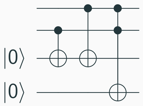
This restricts the set of possible operations, as well. We only have permutations:
In general, given a classical circuit for \(f(x)\), we can obtain
$$
|x\rangle|0\rangle \rightarrow |x\rangle |f(x)\rangle
$$
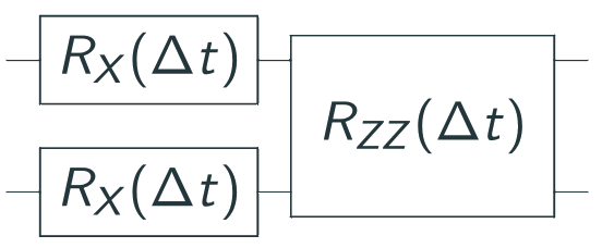
Suzuki-Trotter decomposition
$$ H = {\color{blue}A} + {\color{green}B} $$
Assume we can evolve under \(A\) and \(B\). How to get evolution under \(H\)?
$$
e^{-i H \epsilon} \approx {\color{blue}e^{-i A \epsilon}} {\color{green}e^{-i B \epsilon}}
$$
So, time-evolve by rapidly alternating between two Hamiltonians
$$
e^{-i H t} \approx \left({\color{blue}e^{-i A \epsilon}} {\color{green}e^{-i B \epsilon}}\right)^{t / \epsilon}
$$
Field theories, the finite way
Each lattice site has a degree of freedom with Hilbert space \(\mathcal H_1\). The whole system has Hilbert space
$$
\mathcal H = \mathcal H_1 \otimes \mathcal H_1 \otimes \cdots
$$
Some Hamiltonian \(H\) couples the different lattice sites. For a spin system, we might have
$$
H = \sum_{\langle i j\rangle} \sigma_z(i) \sigma_z(j) + \sum_i \sigma_x(i)
$$
When correlations are large, the lattice structure is irrelevant, hence "field theory".
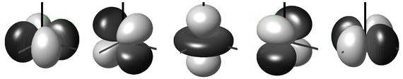
Quantum mechanics on a group
The Hamiltonian of a free particle moving on \(G = SU(3)\):
$$
H = -\nabla_\ell^2
$$
Hilbert space is \(\mathbb C G\), the space of complex functions on \(G\).
When performing time evolution, we would like \( e^{-i H \Delta t} e^{-i H \Delta t} \cdots \), but instead we get:
$$
\color{blue}e^{-i H \Delta t}
\color{red} U_{\mathrm{drift}}
\color{blue}e^{-i H \Delta t}
\color{red} U_{\mathrm{drift}}
\color{blue}e^{-i H \Delta t}
\color{red} U_{\mathrm{drift}}
\cdots
$$
Most states are unphysical.
Changing the Hamiltonian
Suppress unphysical states with an energy penalty.
Define \( H_{\mathrm{gauss}} \) by:
$$
H_{\mathrm{gauss}} |\Psi\rangle = 0
$$
for physical states, and
$$ H_{\mathrm{gauss}} |u\rangle = |u\rangle $$
for unphysical states.
and add \( H_{\mathrm{gauss}} \) to the Hamiltonian used for evolution.
Paths which pass through the unphysical subspace will pick up phase cancellations and be supressed.
But how can we implement \( H_{\mathrm{gauss}} \)?
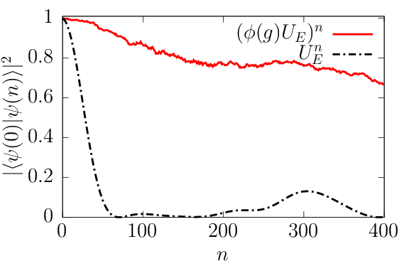
Random gauge transformations
But how can we implement \( H_{\mathrm{gauss}} \)?
We don't need to! We only need \( U_{\mathrm{gauss}} \sim e^{-i H_{\mathrm{gauss}} t} \)
At long times (equivalently, large energies), this gives each unphysical state a random phase. Approximate by performing a random gauge transformation.
$$
e^{-i H \Delta t}
\phi(g_0)
e^{-i H \Delta t}
\phi(g_1)
e^{-i H \Delta t}
\cdots
$$
Each \(\phi(g)\) blesses an unphysical state with a random phase.
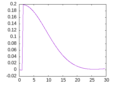
Random gauge transformations: Demonstration
With gauge group \( D_3 \)
Near-term targets?
Inelastic scattering: need a \((4\;\mathrm{fm})^3\) box (at least). (See: Jordan, Lee, Preskill (2011).)
With a lattice spacing of \(0.1\;\mathrm{fm}\), that's \(2 \times 10^5\) links, or \( 2 \times 10^6\) qubits. Yikes!
What can we do with a small volume? Hydrodynamics
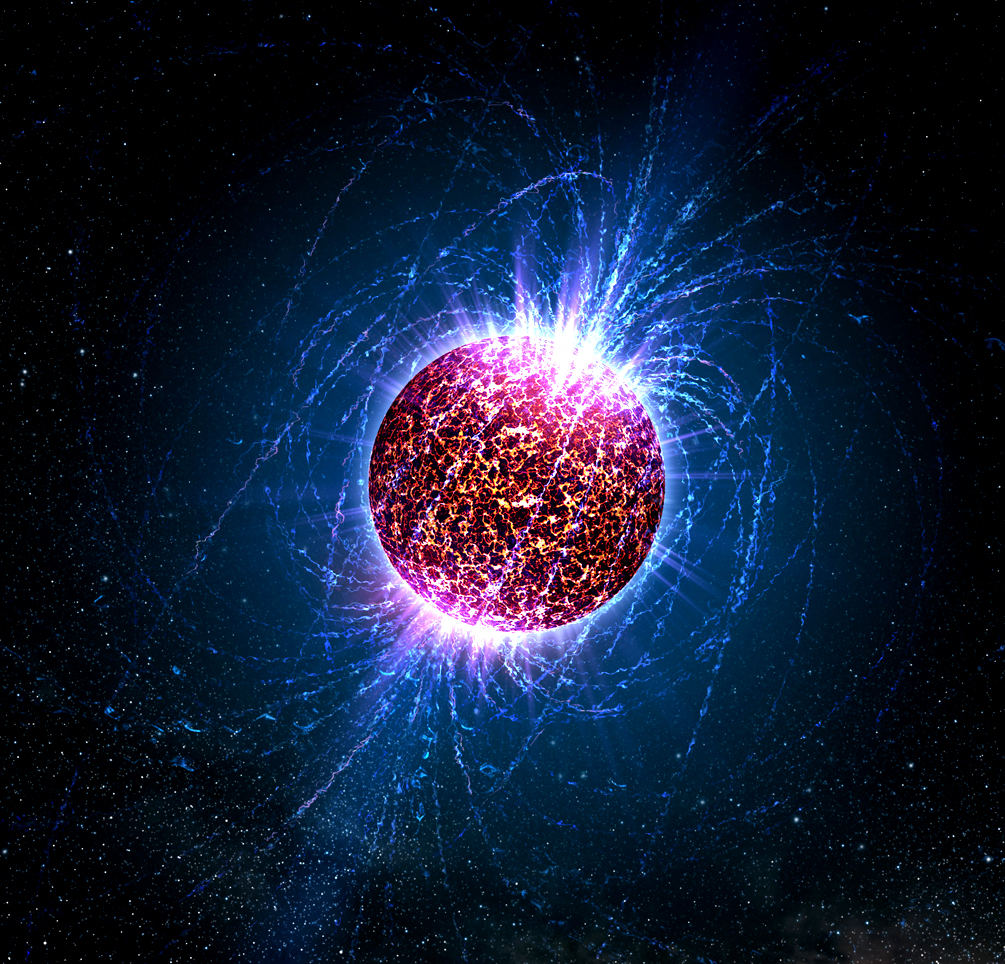
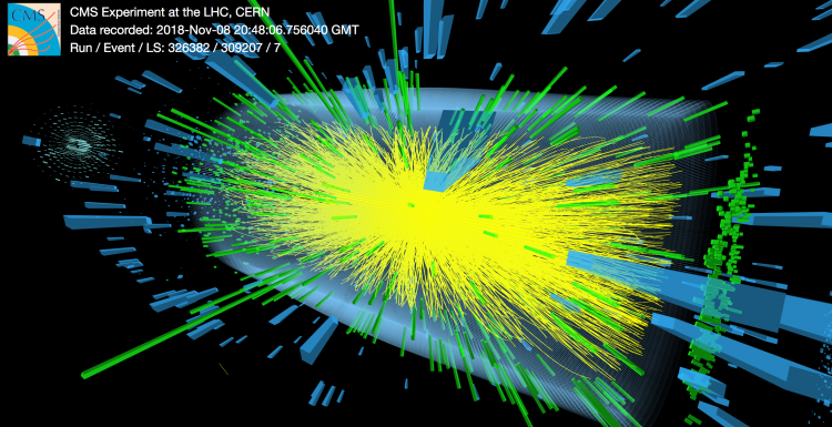
Fireballs
Early in a heavy-ion collision, temperature is \(\sim 300\;\mathrm{MeV}\); physics well-described by hydrodynamics.
$$\def\d{\mathrm{d}}
\rho \frac{\d u_i}{\d t} + \partial_i p = {\color{blue}\eta} \left(\frac 1 3 \partial_i \partial_j u_j + \partial_j^2 u_i \right) + {\color{blue}\zeta}\cdots
$$
The fireball is small (\(\sim 10\;\mathrm{fm}\))! This is good for us: even smaller volumes might behave hydrodynamically.
EFT coefficients (shear viscosity, ...) not known from first principles.
Preparing a thermal state
(The least sophisticated algorithm on the planet.)
Too cold? "Whack and wait".
Too hot? You're on your own.
Advantages: simple, cheap.
Can we go cheaper?
Avoiding state preparation
State preparation dominates the gate cost of the calculation.
Can we skip state preparation?
Classical lattice methods are very good at simulating thermodynamics; can't do real-time.
Quantum computers simulate real-time evolution easily; thermodynamics can be expensive.
Several ways of turning \(\rho\) into a probability distribution to sample. We could take the diagonal
$$
\langle \mathcal O \rangle = \frac{\sum_i \rho_{ii} \mathcal O_{ii}}{\sum_i \rho_{ii}}
$$
Equality holds when \(\mathcal O\) is diagonal. (Common in lattice QCD.)
Therefore: sample pairs of states \(|i\rangle\langle j|\), distributed by \(\rho_{ij}\).
How to compute \(\mathcal O(t)_{ij}\)? This part is done on a quantum computer.
Preparing a basis state \(|i\rangle\) is cheap. Start with the states
$$
|+\rangle = |i\rangle + |j\rangle\;\mathrm{ and }\;
|-\rangle = |i\rangle - |j\rangle
$$
and look at \(\langle + | \mathcal O(t) | +\rangle - \langle - | \mathcal O(t) | -\rangle\).
How to sample
How do we sample \(\rho_{ii}\)?
Even computing \(\rho_{ij}\) is hard! Turns out, sampling is easier:
$$
\mathrm{Tr\,} e^{-\beta H}
=
\sum_{i,j,k,\ldots} \color{green}\left(e^{-\delta H}\right)_{ij} \left(e^{-\delta H}\right)_{jk} \cdots
$$
For small \(\delta\), the summand is easily computed. This is a joint distribution over \((i,j,k,\ldots)\). Marginalized, it approximates \(\rho_{ii}\).
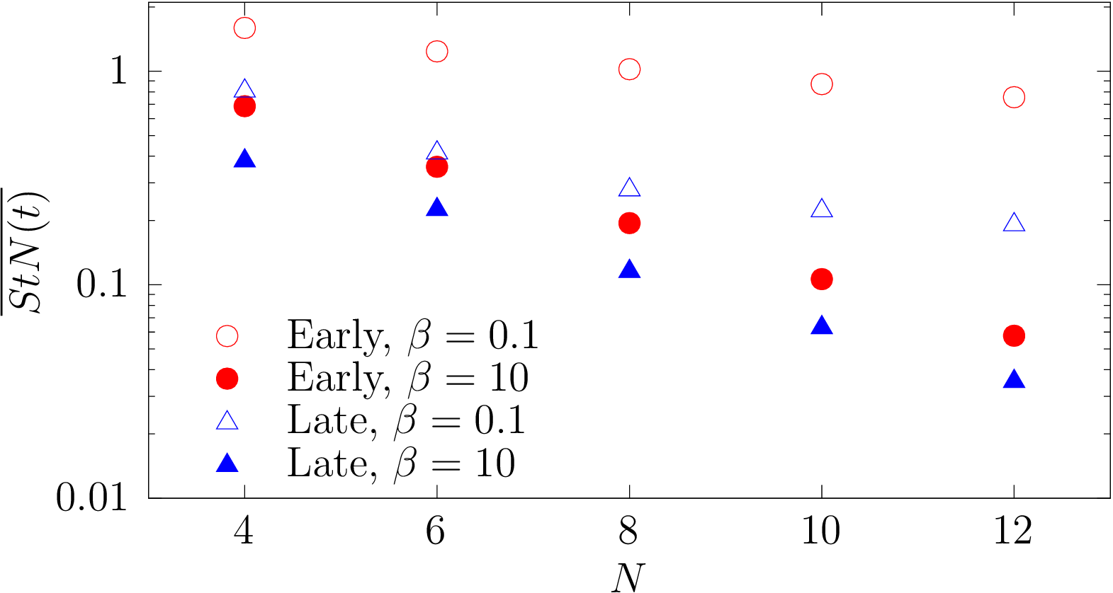
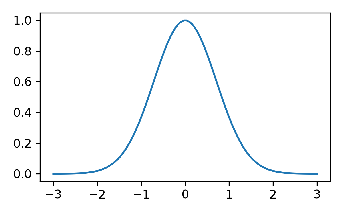
Create a shear wave:
\[
u_x = A \cos(k z)
\]
Near equilibrium, a shear wave decays as
\[
A(t) \sim A(0) e^{-\frac{\eta k^2}{\rho} t}
\]
(Discussed and endorsed by Hess (2001))
Finite volume effects
Classical Approximation
Finite-volume effects set by \(\ell_{\mathrm{mfp}} \sim 0.5\;\mathrm{fm}\). (Not trustworthy!)
Suggests box sizes with \(L \sim 1-2\;\mathrm{fm}\) sufficient!
With a lattice spacing of \(0.2\;\mathrm{fm}\), this is a \(5^3\) to \(10^3\) lattice.
Gauge/Gravity
Using Green-Kubo (\(T^{12}\) channel, there are no finite-volume effects in the \(N_C \rightarrow \infty\) limit of \(\mathcal N=4\) SYM. (This is a holography special.)
In the \(T^{01}\) channel, FV regulated by temperature. Again, the scale is \(\sim 1 \;\mathrm{fm}\).
Stay tuned...
All told, for \(3 + 1\) \(SU(3)\) Yang-Mills, \(\sim 4 \times 10^4\) qubits
For \(2 + 1\) \(SU(2)\) gauge theory, \(\lesssim 1500\) qubits
Hydrodynamics of a (strongly interacting) \(2+1\) spin model could be \(\sim 100\) qubits.


 $$ \int f \approx 1 \pm 0.5$$
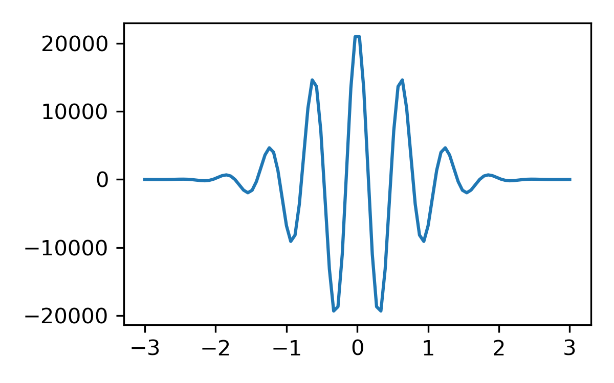 $$ \int f \approx 0 \pm 10^4 $$