• Vector space of states (\(|\psi\rangle\))
• Positive-semidefinite inner product: \(\langle \psi | \psi \rangle \ge 0\)
• Hermitian observables
• Hamiltonian (Hermitian generator of time evolution)
\[ U(t) = e^{-i H t} \]
• Ground state \(|\Omega\rangle\) minimizing \(\langle \Omega | H| \Omega\rangle\)

• Ground state properties
• Thermal properties
• Time-dependent behavior (near or far from equilibrium)

Remember: \({\color{green}\langle \Psi|\color{blue}|\Psi\rangle}\ge 0\)

Of course \({\color{green}\langle 0 | x \color{blue}x | 0 \rangle} \ge 0\) and \({\color{green}\langle 0 | p \color{blue}p | 0 \rangle} \ge 0\). So: \(\langle \hat H \rangle \ge 0\).

We can do better, by using the uncertainty principle: \([x,p] = i\hbar\).

\[ H = - \mu \sigma_x \]

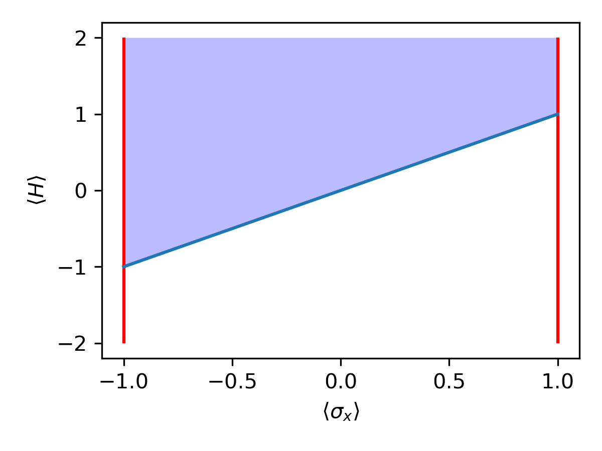
Define \(|\Psi\rangle = (1 + \sigma_x)|0\rangle\) \[ \langle \Psi | \Psi\rangle \ge 0 \Longrightarrow \langle 2 + 2\sigma_x \rangle \ge 0 \Longrightarrow \langle \sigma_x \rangle \ge -1 \]

So \(\langle H\rangle \ge -\mu\) (as expected!)

Let's move from states to operators!

Consider a basis of operators \(\mathcal O_1,\ldots\mathcal O_N\). We can build a matrix \[ M = \left(\begin{matrix} \langle \mathcal O_1^\dagger \mathcal O_1 \rangle & \langle \mathcal O_1^\dagger \mathcal O_2\rangle & \cdots \\ \langle \mathcal O_2^\dagger \mathcal O_1 \rangle & \langle \mathcal O_2^\dagger \mathcal O_2\rangle & \cdots \\ \vdots & \vdots & \ddots \end{matrix}\right) \]

Proof: for any vector \(v\), consider the operator \(\mathcal O = \sum_i v_i \mathcal O_i\). \[ v^\dagger M v = \langle (\vec v \cdot \mathcal {\vec O})^\dagger (\vec v \cdot \mathcal {\vec O}) \rangle = \langle \mathcal O^\dagger \mathcal O \rangle \ge 0 \]

Let \(C\) be an \(N \times N\) matrix. We wish to find a positive semi-definite matrix \(X\) \[ \text{minimizing }\;\mathrm{Tr}\;CX \] subject to linear constraints on the matrix elements of \(X\).

In our context, \(C\) specifies the Hamiltonian, and the linear constraints follow from the commutation relations.

Example: \(\langle xp\rangle - \langle px\rangle = i\hbar\)

Here's a basis of operators: \(\{1, \sigma_x, \sigma_y, \sigma_z\}\). (In fact this basis is complete.)

Note that any assignment of expectation values obeying the above constraint corresponds to some density matrix \(\rho\).

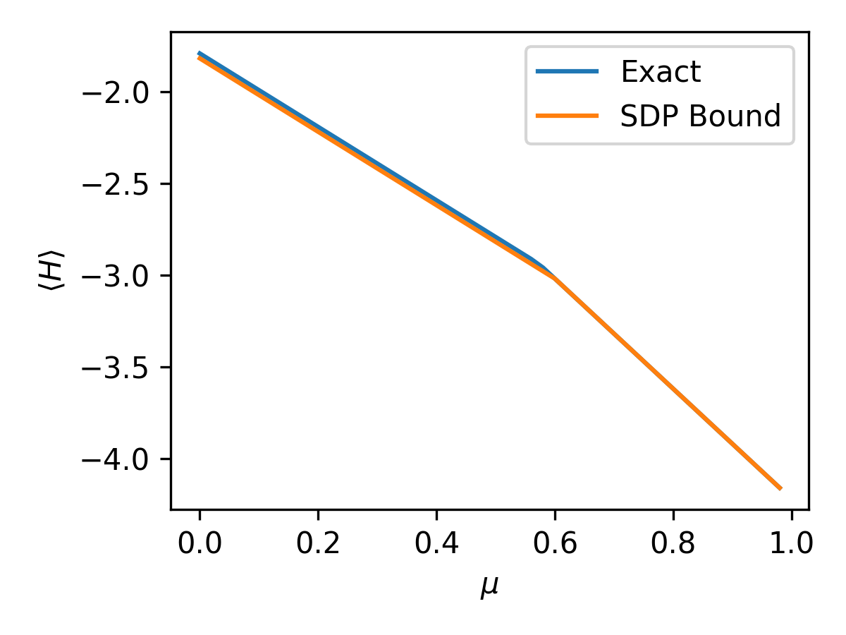
For \(H = -\mu \sigma_x\), only the upper-left \(2\times 2\) minor is needed. \[ \left|\begin{matrix} 1 & \langle \sigma_x \rangle\\ \langle \sigma_x \rangle & 1 \end{matrix}\right|\ge 0 \Longrightarrow 1 - \langle \sigma_x \rangle^2 \ge 0 \]

We can't use a complete basis. Let's start with \(\{1,x,p\}\). \[\color{green} \left(\begin{matrix} 1 & \langle x\rangle & \langle p \rangle\\ \langle x \rangle & \langle x^2 \rangle & \langle xp \rangle\\ \langle p \rangle & \langle xp \rangle + i\hbar & \langle p^2 \rangle \end{matrix}\right)\succeq 0 \]

This is just one small part of the "full" SDP, but it represents several important constraints!

Using the lower \(2\times 2\) minor: \[ \left|\begin{matrix} \langle x^2 \rangle & \langle xp \rangle\\ \langle xp \rangle + i\hbar & \langle p^2 \rangle \end{matrix}\right| = \langle x^2 \rangle \langle p^2\rangle - \langle xp\rangle^2 - i \hbar \langle xp \rangle \ge 0 \Longrightarrow \langle x^2\rangle \langle p^2\rangle \ge \hbar \]

Adding more operators can only make the bound stricter.

In general, if we can write \[ H = C + \mathcal O_1^\dagger \mathcal O_1 + \mathcal O_2^\dagger \mathcal O_2 + \cdots \]

then the bound \(\color{blue}\langle H \rangle \ge C\) follows immediately.

• The space of permitted expectation values is convex
• The ground state sits at the boundary (the lowest possible value of \(\langle H \rangle\))
• Any sum-of-squares representation yields a rigorous lower bound
• Equivalently, solving a truncated SDP yields a rigorous lower bound

Quantum information

Conformal bootstrap: a history lesson

Computational applications (matrix models, lattice field theories)

Setup: Alice samples a random number \(i \in 1\ldots N\), with probability \(p_i\). Alice sends a quantum state \(\rho_i\) to Bob. Bob must make a measurement and guess \(i\).

How well can Bob do?

Bob will measure onto some set of projectors \(\{E_j\}\), and reply \(j\) with probability \[ P_j(|\psi\rangle) = \mathrm{Tr}\; E_j \rho_i \] We want to maximize the success probability, that is \[ \sum_i p_i \mathrm{Tr}\; \rho_i E_i \] subject to \[ E_i \succeq 0 \text{ and } \sum_i E_i = 1 \]

Surprise! It's an SDP!

Alice and Bob each have access to one half of a quantum system. Alice can measure operators \(E_\alpha\), and Bob \(E_\beta\). A quantum correlation is: \[ P_{\alpha\beta} = \mathrm{Tr}\;E_\alpha E_\beta \rho \]

Which probabilities \(P_{\alpha\beta}\) are achievable quantum correlations?

Answer: \(\Gamma_{ij} = \mathrm{Tr}\; S_i^\dagger S_j \rho \succeq 0\). So, we require that such a \(\Gamma\) exists, compatible with the given probabilities (a linear condition). \[\color{green} \mathcal S_1 = \{E_\alpha\} \cup \{E_\beta\} \;\text{ ; }\; \mathcal S_2 = \{E_\mu E_\nu\} \;\text{ ; }\; \cdots \]

Tsirelson's problem: can every quantum correlation be approximated by a system of finite Hilbert space dimension?

No (!)

Finding a global minimum is hard, in general.

For convex functions, it's much easier

Current tools for solving SDPs: SDP-A, MOSEK, SDPB

There is certainly room for improvement in this space.

The original dream: construct an S-matrix purely from symmetries and consistency conditions.

Circumvents the need for a sensible definition of field theory.

Fell out of favor as QCD became understood.

\(\sim 40\) years pass...

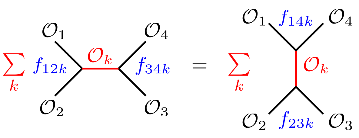
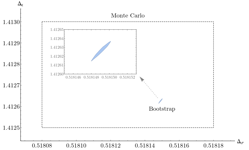
Conformal bootstrap: modern numerical techniques allow the bootstrap program to strongly constrain the space of conformal field theories, purely from symmetries and consistency.

Now "bootstrap" and "semi-definite programming" are somewhat synonymous.

A conformal field theory is:

• Lorentz invariant
• Unitary
• Scale invariant (conjecturally implies conformal invariance)
• Characterized by critical exponents

Why do we care?

At asymptotically high or low energies, any field theory approaches a conformal fixed point.

Also, lamppost effect: we study these because they're (relatively) easy.

To study individual eigenstates, we can impose: \[ \langle H \mathcal O \rangle = E \langle \mathcal O \rangle \]

For the anharmonic oscillator, this yields constraints like:

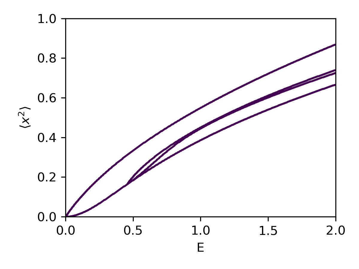
The allowed region is not convex!

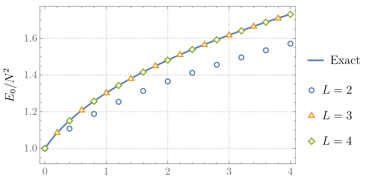
Let \(X,P\) be \(N\times N\) Hermitian matrices of operators, obeying \[ [P_{ij},X_{kl}] = -i \delta_{ik} \delta{jl} \]

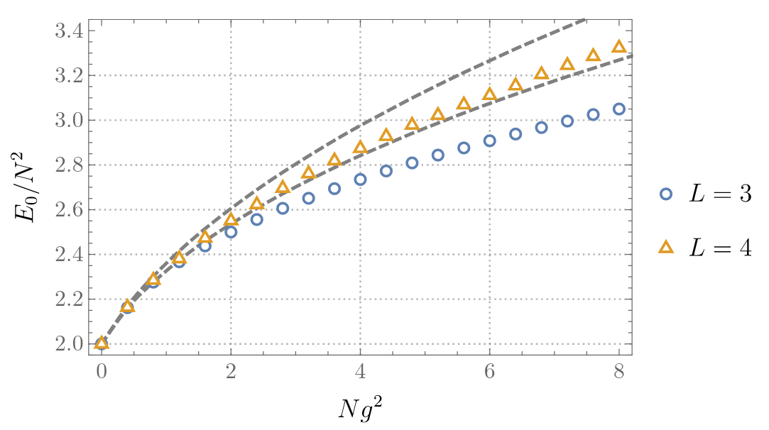
Some Hamiltonians \[ \color{green} H_{\mathrm{easy}} = \mathrm{Tr}\; P^2 + \mathrm{Tr}\;X^2 + \frac{g}{N}\mathrm{Tr}\;X^4 \] \[\color{red} H_{\mathrm{harder}} = \mathrm{Tr}\; P_X^2 + \mathrm{Tr}\; P_Y^2 + m^2 \mathrm{Tr}\;(X^2 + Y^2) - \mathrm{Tr}\;g^2[X,Y]^2 \]

Matrix models are quantum mechanical and consistent.

Conjecture: Larger matrix models (e.g. BFSS) exhibit emergent spacetime.

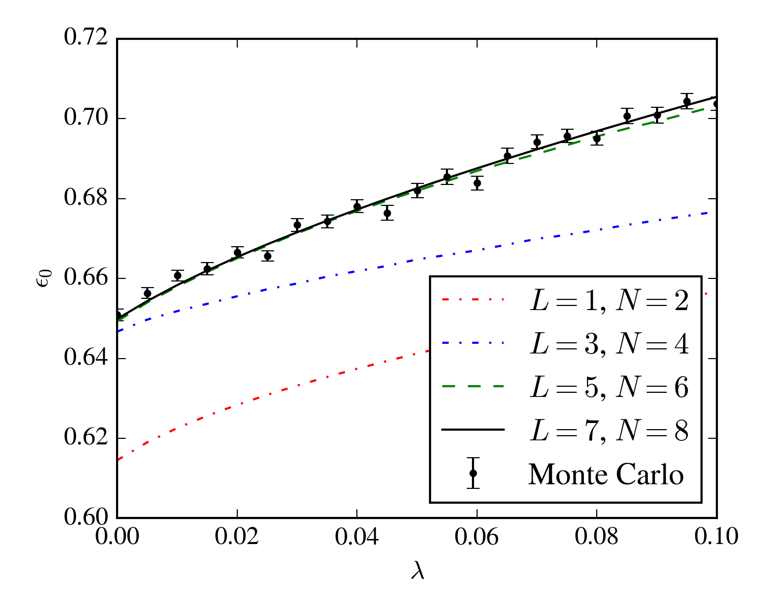
Each lattice site has a degree of freedom with Hilbert space \(\mathcal H_1\). The whole system has Hilbert space $$ \mathcal H = \mathcal H_1 \otimes \mathcal H_1 \otimes \cdots $$

Some Hamiltonian \(H\) couples the different lattice sites. For a spin system, we might have $$ H = \sum_{\langle i j\rangle} \sigma_z(i) \sigma_z(j) + \sum_i \sigma_x(i) $$

When correlations are large, the lattice structure is irrelevant, hence "field theory".

The lattice Thirring model (staggered fermions):

At finite chemical potential, lattice Monte Carlo exhibits the sign problem.

• Operators: all \(\chi(x)\) and \(\chi^\dagger(x)\)
• \(L = 4\)
• \(m = 0.5\)
• \(g^2 = 0.1\)

No evidence of a sign problem