The Easiest Sign Problem

\[ Z = \int d x\; e^{-x^2 - {\color{red}2 i \alpha x}} \] \[\color{blue} Z_Q = \int d x \; e^{-x^2} \]

We must sample with respect to the quenched Boltzmann factor. Observables are computed via \[ \langle \mathcal O \rangle = \frac{\langle\mathcal O e^{-i S_I} \rangle_Q}{\langle e^{-i S_I}\rangle_Q} \]

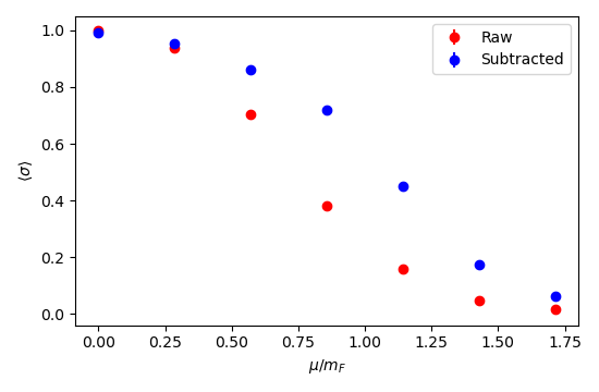
The sign problem is measured by \[ \langle \sigma\rangle \equiv \frac Z {Z_Q} \sim e^{-\alpha^2} \]

Contour Integrals for the Sign Problem

The Boltzmann factor \(e^{-S}\) is complex. Sample with \(e^{-S_R}\) and reweight. \[ \langle\sigma\rangle = \frac{\int e^{-S}}{\int |e^{-S}|} \]

Theorem: the integral of a holomorphic function is unchanged by contour deformation.

Thirring Model

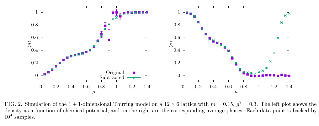
Relativistic fermions in \(1+1\) dimensions with a repulsive 2-body interaction. \[ S_{\mathrm{thirring}} = \frac 1 {2 g^2}\sum_{x,\mu} \big(1 - \cos A_\mu(x)\big)- \frac{N_f}{2} \log \det K[A] \]

The \(N_f=1\) theory is exactly solvable. Strong coupling marked by \(m_B \sim m_F\).

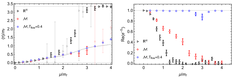
Sign problem exponentially bad in \(m^2 V\).

Finding Contours: Holomorphic Gradient Flow

Evolve every point on the real plane according to the holomorphic gradient flow: \[ \frac{d z}{dt} = \left({\frac{\partial S}{\partial z}}\right)^* \] For short flow times, improves the average sign by decreasing the quenched partition function. (Maximally efficient!) \[ Z_Q = \int dz\, |e^{-S}| \]

Alas, evolving this ODE at every sample is dreadfully slow.

For an \(8^4\) QCD lattice, evaluating the Jacobian determinant requires a \(10^5 \times 10^5\) matrix. (\(\sim 10\) times larger than the Dirac matrix)

Learning Flowed Contours

Algorithm:

Sample many points from flowed manifold.
Train neural network to approximate flow (supervised learning)
Run Monte Carlo using approximated flow.

\[ \mathop{\mathrm{Re}} A = M_3 \sigma[M_2 \sigma(M_1 \mathop{\mathrm{Im}} A)] \]

Downsides:

Determinant computation still required.
Many samples points required to train accurately.
Flowed manifold is not optimal!

Direct Contour Optimization

Evaluating \(\langle \sigma \rangle\) itself is hard. The sign problem manifests as a signal-to-noise problem.

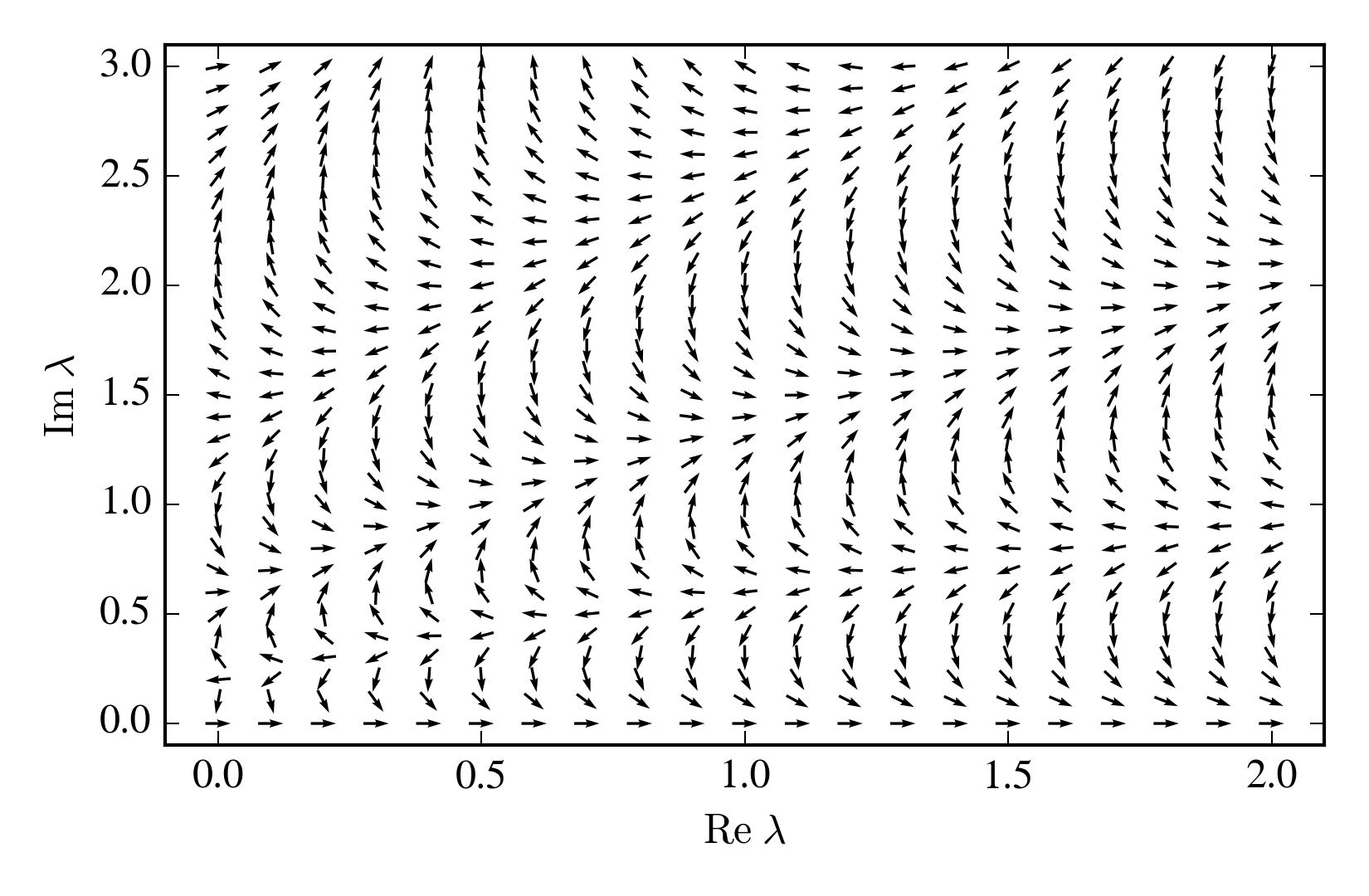
But, we don't need to! We just need to minimize \(Z_Q\), and \[\color{green} \frac{d}{d t}\lambda = - \frac{\partial}{\partial \lambda} \log Z_Q \] has the form of a quenched (i.e., sign-free) observable!

This isn't complex analysis---it's a general principle. Contour deformations:

Leave \(Z\) alone, while
Potentially modifying \(Z_Q\).

Any strategy with those properties can be optimized in the same way.

Early Success: Thirring Model

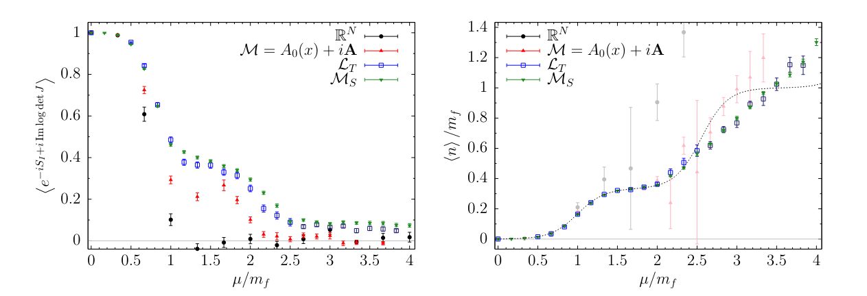
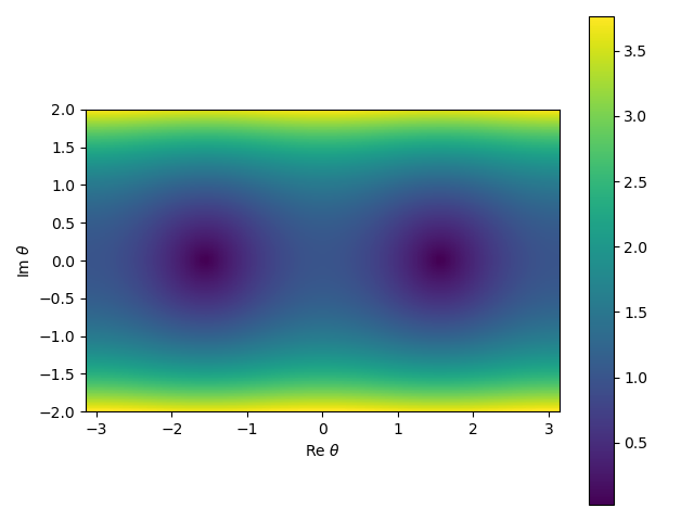
Best results obtained with a simple ansatz, rather than a deep neural network: \[ \mathop{\mathrm{Im}} A_0(x) = a + b \cos \mathop{\mathrm{Re}} A_0(x) + c \cos \mathop{\mathrm{Re}} 2 A_0(x) \]

Another Perspective: Normalizing Flows

Goal: sample from \(p(z)\)

A normalizing flow is a map \(\phi\) \[ \int_{-\infty}^x e^{-x^2} dx = \int_{-\infty}^{\phi(x)} p(z)\, dz \]

Sample from the Gaussian, then apply \(\phi\).

(Any easily sampled distribution can replace the Gaussian.)

What if \(\phi(x)\) is complex?

Complex normalizing flow \(\Rightarrow\) contour deformation

A complex normalizing flow gives a locally perfect contour deformation

Analytic Continuation of Normalizing Flows

Here's a normalizing flow for scalar field theory:

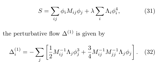
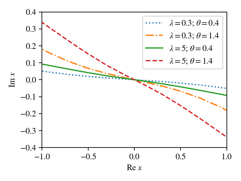
What if \(M,\Lambda\) are complex? Doesn't matter; still a good normalizing flow.

Normalizing flows are analytic in action parameters

To summarize:

Normalizing flows always exist for real distributions (theorem)
These can be analytically continued for complex parameters (ideology)
Complex normalizing flow gives (locally perfect) integration contour

Scalar Field Theory at Complex Coupling

\[ S = \int dx\, \frac 1 2 \left(\frac{\partial\phi}{\partial x}\right)^2 + \frac {m^2}{2} \phi(x)^2 + \lambda \phi(x)^4 \]

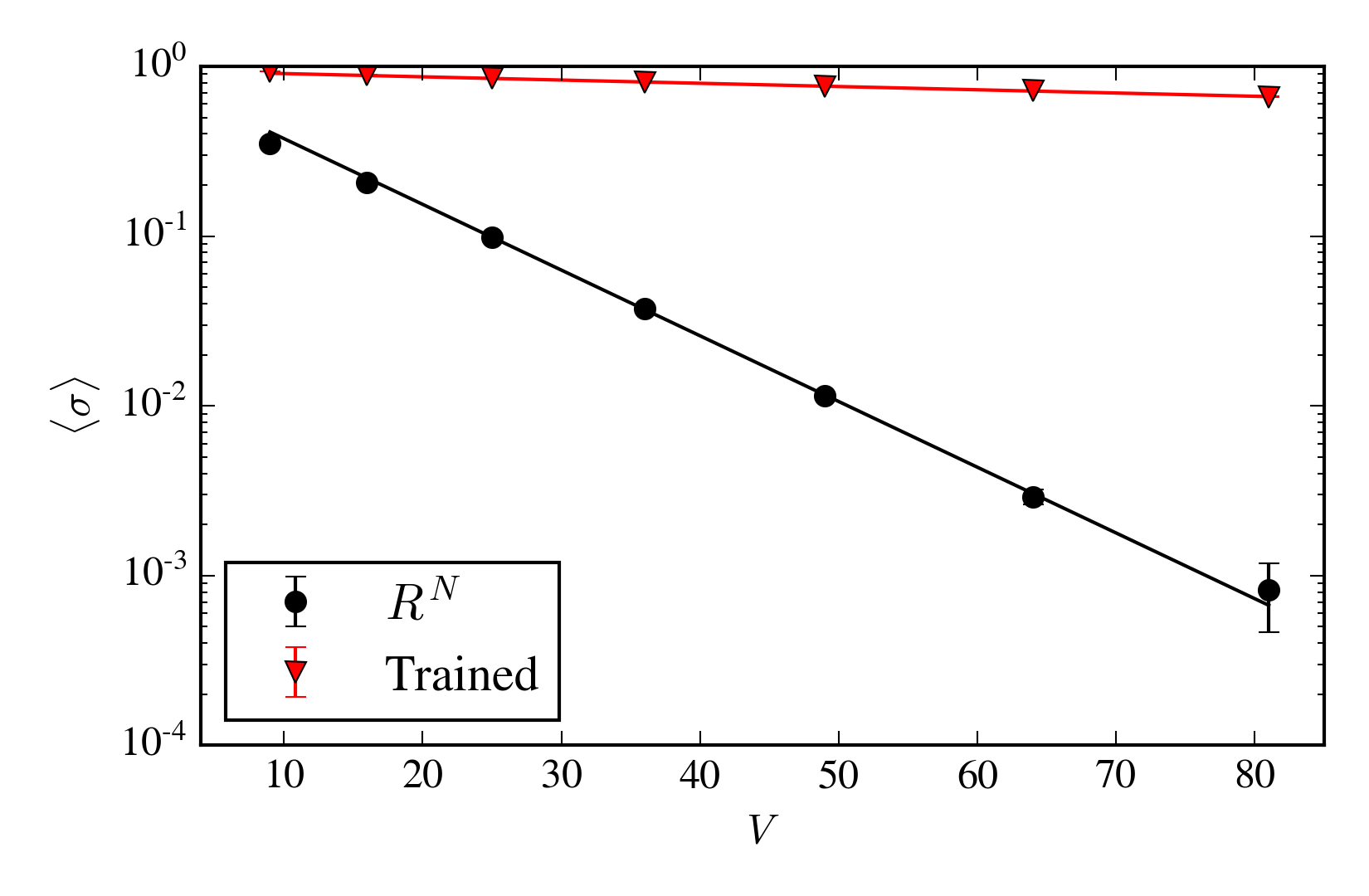
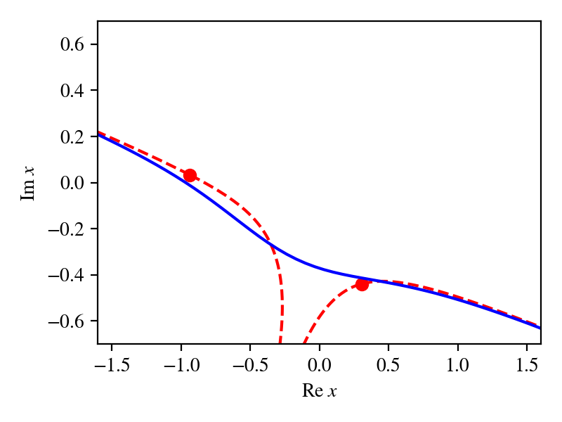
At \(\mathop{\mathrm{Im}}\lambda \ne 0\), this model has a sign problem. Train a contour as before, and the sign problem nearly disappears:

Cost Function for Normalizing Flows

\begin{align} C_{\mathrm{nf}}(\lambda) &= \Bigg\langle\bigg|\underbrace{\frac{\phi^2}{2} - \Re\log\mathcal N - \Re S(\tilde\phi_\lambda(\phi)) - \Re \log \frac{\partial\tilde\phi_\lambda}{\partial\phi}}_{\Re (S_{\mathrm{induced}} - S)}\bigg|^2\Bigg\rangle_n\\ &+ \Bigg\langle\bigg|1-\underbrace{\Big(\mathop{\mathrm{csgn}} \frac{\partial \tilde\phi_\lambda}{\partial \phi}\Big)e^{-i\Im \left(S(\tilde\phi_\lambda(\phi)) + \Im \log \mathcal N\right)}}_{e^{-i \Im \left(S_{\mathrm{induced}} - S\right)}}\bigg|^2\Bigg\rangle_n \text. \end{align}

Adiabatic training: Start at real \(\lambda\) and rotate \(\lambda\) while tracking a "good" contour (or normalizing flow).

Analytically Continued Scalar Field Theory

\[ Z(\lambda) = \int \mathcal D\phi\, e^{- (\cdots + \lambda \int \phi^4)} \]

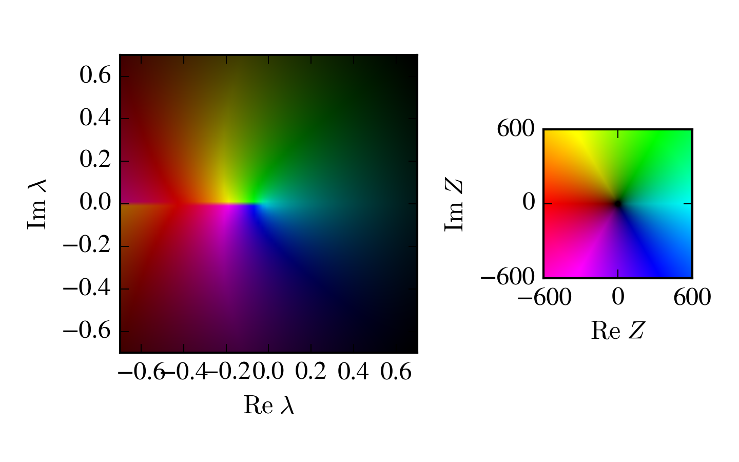
For \(\mathop{\mathrm{Re}}\lambda < 0\) the partition function can be defined only by analytic continuation. This is a "worse than infinitely bad sign problem".

Do Perfect Contours Exist?

Wanted: a manifold such that \[ \left|\int e^{-S} \;d z\right|=\int \left|e^{-S} \;dz\right| \]

This does not automatically solve the sign problem!

Perfect manifolds might be hard to find
Hard to sample from
Observables may have signal-to-noise problem

Example With No Perfect Manifold

\[ Z = \int (\cos \theta + \epsilon) \;d \theta\]

\[Z = 2 \pi \epsilon\]

Quenched partition function is \(O(1)\)

Similar methods reveal that no manifold exists for the mean-field Thirring model.

Directly Modifying the Boltzmann Factor

Modify the partition function by subtracting any function \(g(\phi)\) that integrates to \(0\)

\[ Z = \int d\phi\,e^{-S(\phi)} \rightarrow \int d\phi\,\left( e^{-S(\phi)} - g(\phi) \right)\]

Physics (the partition function as a function of various sources) is unchanged, but the sign problem...

\[ Z_Q = \int \left|e^{-S(\phi)}\right| \ne \int \left|e^{-S(\phi)} - g(\phi)\right| = \tilde Z_Q \]

All contour deformations are subtractions: \(\int d\phi\, f(\phi) - f(\tilde\phi(\phi)) = 0\)

Perfect Subtractions Exist

For any sign problem, a subtraction exists that removes it.

\[g(\phi) = e^{-S(\phi)} - \frac{\int d\phi\,e^{-S(\phi)}}{\int d\phi} \]

This is not unique, but it is "close" to unique. Adding a generic function \(\tilde g \sim e^{-S}\) breaks the subtraction. Adding a generic function \(\tilde g \sim Z_Q\) is okay.

General trick to obtain functions that integrate to \(0\): \(g(\phi) = \frac{\partial}{\partial \phi_i} v_i\). (Almost useful for machine learning, but \(v \sim e^{-S}\) is required.)

Perturbative Subtractions

Any systematic expansion can be used to obtain a subtraction.

Heavy-dense limit: a lattice expansion in large \(\mu\): \[ \det K[A] = {\color{blue}2^{-\beta V} e^{\beta V \mu + i \sum_x A_0(x)}} + O(e^{\beta (V-1) \mu}) \]

Learning Subtractions

\[ Z = \int e^{-S} \rightarrow \int e^{-S}\left(1 - v \cdot \nabla S + \nabla \cdot v\right) \]

This form of subtraction is the same, at leading order in \(v\), as performing an infintesimal contour deformation.

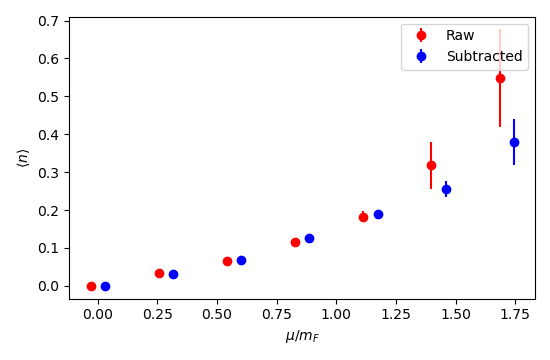
\[ \langle \mathcal O\rangle = \frac{\int e^{-S} \mathcal O}{\int e^{-S}} \rightarrow \frac{\int e^{-S} \left(1 - v \cdot \nabla S + \nabla \cdot v\right) \left(\mathcal O - \frac{v \cdot \nabla \mathcal O}{\left(1 - v \cdot \nabla S + \nabla \cdot v\right) }\right) }{\int e^{-S}\left(1 - v \cdot \nabla S + \nabla \cdot v\right) } \]

Other procedures for measuring observables generally result in terrible signal-to-noise.

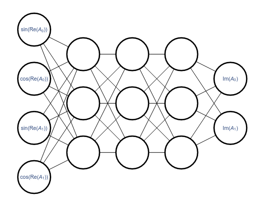
Training a 2-layer network on a 6-by-6 lattice with \(m_B = 0.33(1)\), \(m_F=0.35(2)\):

Does this trick (meaningfully) undermine the existence guarantees?

Machines Learning to Solve Sign Problems