QCD is a non-perturbative theory. (There's no small parameter about which to Taylor expand.)
At every link lives a unitary matrix.
$$ U_{yx} \in SU(3) $$
The action is a sum over all `plaquettes'.
$$
S = \sum_P \mathrm{Re\,Tr\,} P
$$
This is a theory of with a finite number of degrees of freedom. Expectation values are given by:
$$ \left<\mathcal O\right> = \frac{\int \mathcal D U\;e^{-S[U]} \mathcal O[U]}{\int \mathcal D U\;e^{-S[U]}}$$
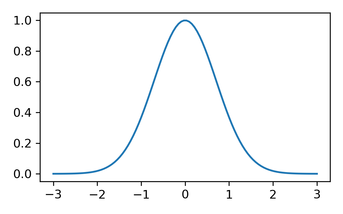
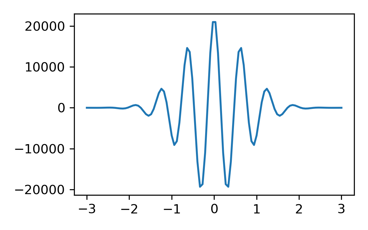
A sign problem
$$ \int f \approx 1 \pm 0.5$$
$$ \int f \approx 0 \pm 10^4 $$
$$
\langle x_1|e^{-i H t}|x_0\rangle = \int_{x(0)=x_0}^{x(1)=x_1} \mathcal D x(t) \;e^{i S[x]}
$$
\(x(t)\)
\(\mathrm{Re\,}e^{iS[x]}\)
What calculations have a sign problem?
Calculations that have sign problems:
Real-time response (as opposed to thermal equilibrium)
Hubbard model away from half-filling
Finite density of relativistic fermions
Closely related, but mild: determining the mass of a proton
Calculations without sign problems:
Zero-fermion-density equation of state
Some masses (pion)
Overview
The best model of a quantum system is another quantum system.
Norbert Wiener, almost
A quantum computer is a quantum system evolved in real-time.
Set up an analogy between the quantum computer and the system to be simulated, and treat the computer like a (perfectly controlled) laboratory.
What's the Hilbert space?
$$
\mathcal H = \mathcal H_1 \otimes \cdots \otimes \mathcal H_1
\;\text{ where }
\mathcal H_1 = \mathrm{span}\{|0\rangle,|1\rangle\}
$$
In other words, superpositions of all possible bitstrings.
$$
\mathcal H = \mathrm{span}\{|00\cdots\rangle,|10\cdots\rangle,|01\cdots\rangle,\cdots\}
$$
These fundamental gates are sufficient to construct any unitary we want.
Measurement
In principle, we measure any Hermitian operator. In practice, we measure \(\sigma_z\) acting on each qubit.
$$\Psi = \alpha|0\rangle + \beta|1\rangle$$
Each measurement yields \(1\) or \(0\). Probability of \(1\) is \(\langle\Psi|1\rangle\langle 1|\Psi\rangle = |\beta|^2\).
Thus, we require many measurements for a precise result. This is "shot noise".
Hermitian operators are exactly those which may appear as terms in the Hamiltonian.
State of the art
Current best: \(\sim 50\) qubits.
Each qubit can undergo \(\lesssim 10\) operations before decohering.
Are large processors worth it?
What is a classical computer?
A quantum computer constantly being measured
\(|01\rangle\) is okay; \(\left[|10\rangle + |01\rangle\right]\) gets destroyed
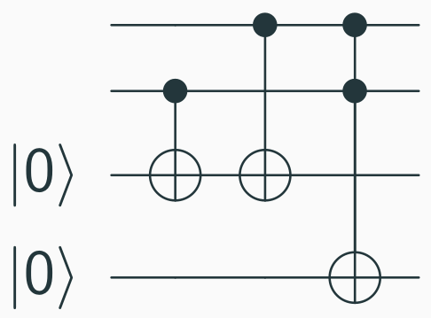
This restricts the set of possible operations, as well. We only have permutations:
In general, given a classical circuit for \(f(x)\), we can obtain
$$
|x\rangle|0\rangle \rightarrow |x\rangle |f(x)\rangle
$$
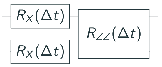
Suzuki-Trotter decomposition
$$ H = {\color{blue}A} + {\color{green}B} $$
Assume we can evolve under \(A\) and \(B\). How to get evolution under \(H\)?
$$
e^{-i H \epsilon} \approx {\color{blue}e^{-i A \epsilon}} {\color{green}e^{-i B \epsilon}}
$$
So, time-evolve by rapidly alternating between two Hamiltonians
$$
e^{-i H t} \approx \left({\color{blue}e^{-i A \epsilon}} {\color{green}e^{-i B \epsilon}}\right)^{t / \epsilon}
$$
Field theories, the finite way
Each lattice site has a degree of freedom with Hilbert space \(\mathcal H_1\). The whole system has Hilbert space
$$
\mathcal H = \mathcal H_1 \otimes \mathcal H_1 \otimes \cdots
$$
Some Hamiltonian \(H\) couples the different lattice sites. For a spin system, we might have
$$
H = \sum_{\langle i j\rangle} \sigma_z(i) \sigma_z(j) + \sum_i \sigma_x(i)
$$
When correlations are large, the lattice structure is irrelevant, hence "field theory".
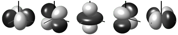
Quantum mechanics on a group
The Hamiltonian of a free particle moving on \(G = SU(3)\):
$$
H = -\nabla_\ell^2
$$
Hilbert space is \(\mathbb C G\), the space of complex functions on \(G\).
$$
H = \sigma_x(a) + \sigma_x(b) + \sigma_z(a) \sigma_z(b)
$$
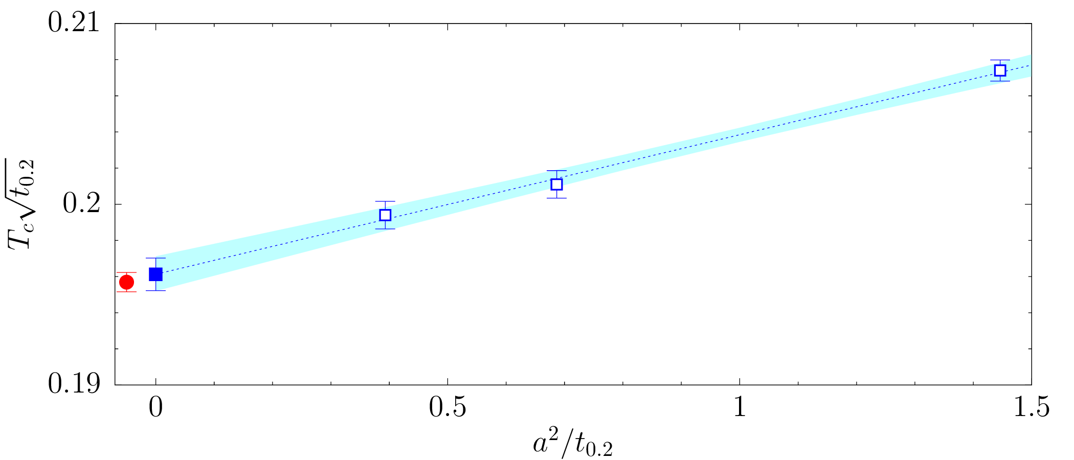
Valentiner gauge theory
We'd like to simulate \(SU(3)\), but \(\mathbb C SU(3)\) is infinite-dimensional.
\[ \color{red}2^Q < \infty \]
We can approximate \(SU(3)\) by a finite subgroup.
\[ S(1080) < SU(3) \]
Is this approximation any good?
After adding an extra term to the action...
$$
S=-\sum_p \left(\frac{\beta_0}{3}\mathrm{Re\,Tr\,} U_p +\beta_1\mathrm{Re\,Tr\,} U_p^2\right)
$$
Construct a dimensionless quantity from: Wilson flow, critical temperature
Particle masses not yet measured...
Maybe
Gauge invariance
The physical Hilbert space is not \(\mathbb C S(1080) \otimes \mathbb C S(1080) \otimes\cdots\).
But, the Hilbert space on the quantum computer is isomorphic to that space!
Time evolution is gauge-invariant.
$$ [P, H] = 0 $$
If we start in a gauge-invariant state, we stay gauge-invariant.
The hadronic tensor
\[
W^{\mu\nu}(q)
=
\int {\mathrm d}x\;e^{iqx}
\left<e^{i H x^0}J^\mu(\vec x) e^{-i H x^0}J^\nu(\vec 0)\right>_{\mathrm{proton}}
\]
The hadronic tensor captures nonperturbative (in QCD coupling) information about the proton. For electron-proton scattering, to leading order in \(\alpha_{\mathrm{QED}}\):
\[
\frac{{\mathrm d}^2\sigma}{\mathrm{d} x\;\mathrm{d} y} = \frac{\alpha^2 y}{Q^4} L_{\mu\nu} W^{\mu\nu}
\]
Preparing an interesting state
Naive state preparation: couple to a heat bath and cool the system. Expensive!
Alternative: adiabatic state preparation
Other proposals:
Tensor networks
Spectral comb (arXiv:1709.08250)
Hybrid state preparation (PhysRevLett 121 170501, 1908.07051)
Hard to analyze, impossible to test
Adiabatic theorem
Take a time-varying (slowly) Hamiltonian \(H(t)\).
Prepare an eigenstate of \(H(0)\), with a gap of \(\Delta\).
When \(\dot H / \Delta^2 \ll 0\), time-evolution will keep us in the eigenstate.
Time needed to prepare ground state: \(\Delta^{-2}\)
Making a proton
Restrict to a certain sector of Hilbert space:
Gauge-invariant states
Zero total momentum
Baryon number 1
Free fermions and glue (massive)
Ground state exactly prepared
Small gap (\(O(\frac 1 V)\))
Hadrons
Large gap (\(m_\pi\))
Total circuit size: \(O(V^3)\)
Measuring the hadronic tensor
\[
W^{\mu\nu}(q)
=
\int {\mathrm d}x\;e^{iqx}
\left<e^{i H x^0}J^\mu(\vec x) e^{-i H x^0}J^\nu(\vec 0)\right>_{\mathrm{proton}}
\]
How do we measure \(e^{i H t}J_0(x)e^{-i H t} J_0(0)\)?
\[
H(t) = H_0 + \epsilon \delta(t) J^\nu(\vec 0)
\]
Linear response: differentiate with respect to \(\epsilon\)
\[
\frac{\partial}{\partial \epsilon} \langle e^{i H t} J^\mu(\vec x) e^{-i H t}\rangle
\]
Several ways of turning \(\rho\) into a probability distribution to sample. We could take the diagonal
$$
\langle \mathcal O \rangle = \frac{\sum_i \rho_{ii} \mathcal O_{ii}}{\sum_i \rho_{ii}}
$$
Equality holds when \(\mathcal O\) is diagonal. (Common in lattice QCD.)
Therefore: sample pairs of states \(|i\rangle\langle j|\), distributed by \(\rho_{ij}\).
How to compute \(\mathcal O(t)_{ij}\)? This part is done on a quantum computer.
Preparing a basis state \(|i\rangle\) is cheap. Start with the states
$$
|+\rangle = |i\rangle + |j\rangle\;\mathrm{ and }\;
|-\rangle = |i\rangle - |j\rangle
$$
and look at \(\langle + | \mathcal O(t) | +\rangle - \langle - | \mathcal O(t) | -\rangle\).
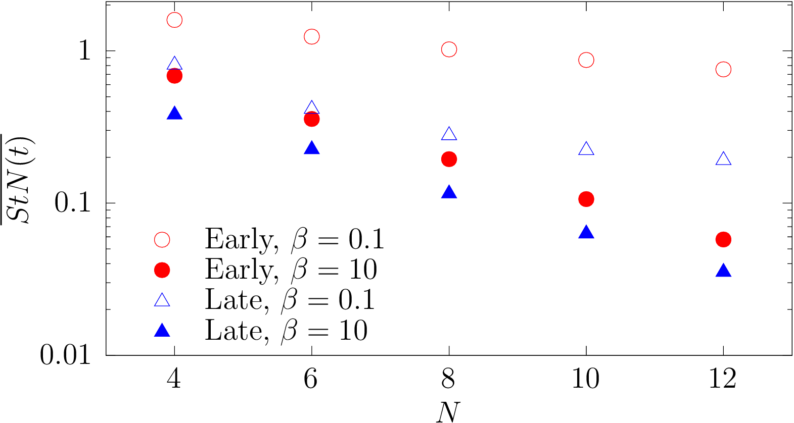
How to sample
How do we sample \(\rho_{ii}\)?
Even computing \(\rho_{ij}\) is hard! Turns out, sampling is easier:
$$
\mathrm{Tr\,} e^{-\beta H}
=
\sum_{i,j,k,\ldots} \color{green}\left(e^{-\delta H}\right)_{ij} \left(e^{-\delta H}\right)_{jk} \cdots
$$
For small \(\delta\), the summand is easily computed. This is a joint distribution over \((i,j,k,\ldots)\). Marginalized, it approximates \(\rho_{ii}\).


 $$ \int f \approx 1 \pm 0.5$$
 $$ \int f \approx 0 \pm 10^4 $$