How should we think about risk mitigation, when investing? Let’s look at a concrete example. I have $100. I’m offered a chance to invest — as much of my money as I’d like. On average, let’s say I’ll gain 10% after a year. But that’s an average. The investment could gain 120%, or lose everything, with equal probability. If I invest everything I’ve got, then the expected value of my investment is good ($10), but of course half the time I’ll be dead broke at the end. Most people would not make such a bet. More sensible is to invest much less, maybe $10. Now the expected value is only $1, but the worst-case scenario is more tolerable. Most people would take this bet without hesitation.

A minor paradox lies here: why do we prefer the lower expected value? A common way around this paradox is to assert that my utility function is logarithmic, not linear, in my wealth. A little arithmetic reveals that betting everything I have (risking an infinitely large loss) now has negative expected value (as measured by my new, logarithmic utility function), while a very small bet retains positive expected value (because \(\log x\) is approximately linear about any \(x>0\)). This is the usual, and fundamentally psychological, story of risk management in investing. The best word to describe it is “wrong”.

There are two things missing from that story. First, the cost of a loss is not limited to the amount of money lost. The lost money is now unavailable for use in the next round of investing — and the next, and the next. To appropriately value the loss, we must take into account the full loss of opportunity. Going broke isn’t just psychologically bad, it’s actually bad, because “broke” is the unique state from which there is no coming back.

Second, the whole notion of “expected value” is somewhat flawed. We don’t have access to many samples from one probability distribution (which is the scenario expected value describes); we have access to exactly one sample. This is the distinction between an average-over-time and an average-over-instances. The former is what you, an individual, have direct access to. The latter is what “expected value” refers to. (We could profitably take the maximally aggressive investment strategy if only we had direct access to an average-over-instances instead of an average-over-time. This is also what insurance contracts can approximate.)

Since we don’t have access to an average-over-instances, we must synthesize one by investing smaller amounts over many rounds. Let’s return to the original example, and this time, assume that there are many rounds of investing. If, on each round, I invest all my money, then I am nearly certain to be broke at the end. (With \(N\) rounds, my probability of being not-broke is \(2^{-N}\).) If I invest an infinitesimal amount each time, then the expected value takes over (central limit theorem-style), and the account grows deterministically, but slowly. Somewhere in between is an optimal rate of growth.

In the real world, multiple strategies are available, and some mixture is going to be optimal. Some strategies may be available for only a limited time. This gets complicated quickly. The core principle, that must not be forgotten, is that the cost of a dollar isn’t the dollar: it’s that dollar, plus all the dollars that dollar would beget. Taking this principle seriously, we hear the echoes of the no-longer-psychological logarithmic utility function. Every dollar has a (meaningless?) “infinite” value as measured in future-dollars. But, with a constant average rate of return, we can ask how far forward or backwards in time an event moves us. At a 10% annual rate of return, a stroke of luck where we double our money moves us forward one year. Losing all our money moves us backwards an infinite amount. This is not just psychological!

Of course, the cost of a lost dollar depends on what strategy is chosen — what a mess! The easiest (and most nearly fool-proof) way to sort through all of this is to run some Monte Carlo simulations to see what growth rate different strategies result in. Before bothering to make a histogram, you get pictures like this: 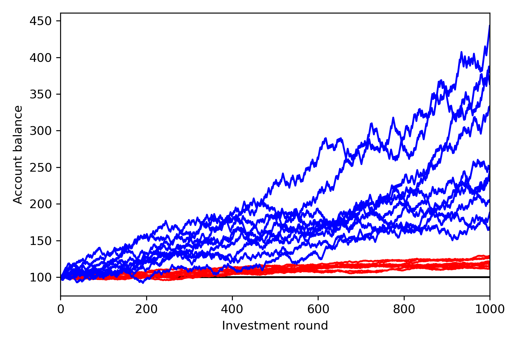Here, blue is the more aggressive strategy (1% invested in the bet above, each round). It is “riskier” in some sense than the more conservative red strategy (0.2% invested each round). However, note that not only is the average higher, so is the worst (likely) scenario. Only the extreme low tail, not likely to be sampled in the Monte Carlo, is worse than the conservative strategy.

Run some Monte Carlo simulations to see the long-term effect of a strategy. This is necessary at any time, but particularly when “exponential growth” is on the table — the results may surprise you! That is the whole of Spitznagel; the rest is commentary; go and learn it.